Dependence of $F_{\rm P}(n)$ on the order $\ell$ of DFA

Another factor that affects the rms fluctuation function of the power-law trend $F_{\rm P}(n)$, is the order $\ell$ of the DFA method used. We first take into account that:

(1) for integer values of the power $\lambda$, the power-law trend $u(i)=A_{\rm P} i^{\lambda }$ is a polynomial trend which can be perfectly filtered out by the DFA method of order $\ell > \lambda$, and as discussed in Sec. 3.2 and Sec. 5.1 [see Fig. 11(b) and (c)], there is no scaling for $F_{\rm P}(n)$. Therefore, in this section we consider only non-integer values of $\lambda$.

(2) for a given value of the power $\lambda$, the effective exponent $\alpha _{\lambda }$ can take different values depending on the order $\ell$ of the DFA method we use [see Fig. 11] -- e.g. for fixed $\lambda > \ell -0.5$, $\alpha _{\lambda } \approx \ell +1$. Therefore, in this section, we consider only the case when $\lambda <\ell -0.5$ (Region II and III).

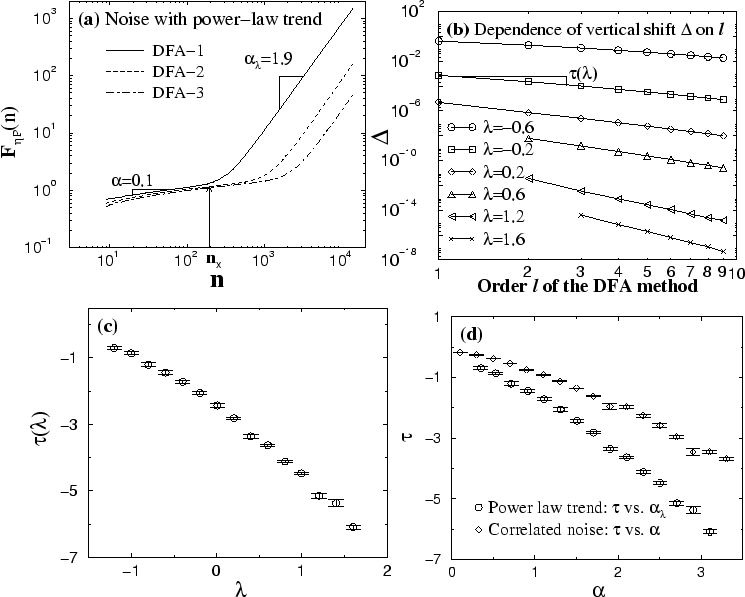
Figure 12: Effect of higher order DFA-$\ell$ on the rms fluctuation function $F_{\rm \eta P}(n)$ for correlated noise with superimposed power-law trend. (a) $F_{\rm \eta P}(n)$ for anticorrelated noise with correlation exponent $\alpha =0.1$ and a power-law $u(i)=A_{\rm P} i^{\lambda}$, where $A_{\rm P}=25/\left(N_{max}\right)^{0.4}$, $N_{max}=2^{17}$ and $\lambda =0.4$. Results for different order $\ell =1,2,3$ of the DFA method show (i) a clear crossover from a region at small scales where the noise dominates $F_{\rm \eta P}(n) \approx F_{\rm \eta}(n)$, to a region at larger scales where the power-law trend dominates $F_{\rm \eta P}(n) \approx F_{\rm P}(n)$, and (ii) a vertical shift $\Delta$ in $F_{\rm \eta P}$ with increasing $\ell$. (b) Dependence of the vertical shift $\Delta$ in the rms fluctuation function $F_{\rm P}(n)$ for power-law trend on the order $\ell$ of DFA-$\ell$ for different values of $\lambda$: $\Delta \sim \ell ^{\tau (\lambda )}$. We define the vertical shift $\Delta$ as the y-intercept of $F_{\rm P}(n)$: $\Delta \equiv F_{\rm P}(n=1)$. Note, that we consider only non-integer values for $\lambda$ and that we consider the region $\lambda <\ell -0.5$. Thus, for all values of $\lambda$ the minimal order $\ell$ that can be used in the DFA method is $\ell >\lambda +0.5$. e.g. for $\lambda =1.6$ the minimal order of the DFA that can be used is $\ell =3$ (for details see Fig. 11(b)). (c) Dependence of $\tau$ on the power $\lambda$ (error bars indicate the regression error for the fits of $\Delta (l)$ in (b)). (d) Comparison of $\tau (\alpha _{\lambda })$ for $F_{\rm P}(n)$ and $\tau (\alpha )$ for $F_{\rm \eta}(n)$. Faster decay of $\tau (\alpha _{\lambda })$ indicates larger vertical shifts for $F_{\rm P}(n)$ compared to $F_{\rm \eta}(n)$ with increasing order $\ell$ of the DFA-$\ell$.

Since higher order DFA-$\ell$ provides a better fit for the data, the fluctuation function $Y(i)$ (Eq. (3)) decreases with increasing order $\ell$. This leads to a vertical shift to smaller values of the rms fluctuation function $F(n)$ (Eq. (4)). Such a vertical shift is observed for the rms fluctuation function $F_{\rm\eta }(n)$ for correlated noise (see Appendix 7.1), as well as for the rms fluctuation function of power-law trend $F_{\rm P}(n)$. Here we ask how this vertical shift in $F_{\rm\eta }(n)$ and $F_{\rm P}(n)$ depends on the order $\ell$ of the DFA method, and if this shift has different properties for $F_{\rm\eta }(n)$ compared to $F_{\rm P}(n)$. This information can help identify power-law trends in noisy data, and can be used to differentiate crossovers separating scaling regions with different types of correlations, and crossovers which are due to effects of power-law trends.

We consider correlated noise with a superposed power-law trend, where the crossover in $F_{\rm\eta P}(n)$ at large scales $n$ results from the dominant effect of the power-law trend -- $F_{\rm\eta P}(n) \approx F_{\rm P}(n)$ (Eq. (18) and Fig. 10(a)). We choose the power $\lambda<0.5$, a range where for all orders $\ell$ of the DFA method the effective exponent $\alpha _{\lambda }$ of $F_{\rm P}(n)$ remains the same -- i.e. $\alpha _{\lambda }=\lambda +1.5$ (region II in Fig. 11(b)). For a superposition of an anticorrelated noise and power-law trend with $\lambda =0.4$, we observe a crossover in the scaling behavior of $F_{\rm\eta P}(n)$, from a scaling region characterized by the correlation exponent $\alpha =0.1$ of the noise, where $F_{\rm\eta P}(n) \approx F_{\rm\eta }(n)$, to a region characterized by an effective exponent $\alpha_{\lambda}=1.9$, where $F_{\rm\eta P}(n) \approx F_{\rm P}(n)$, for all orders $\ell =1,2,3$ of the DFA-$\ell$ method [Fig. 12(a)]. We also find that the crossover of $F_{\rm\eta P}(n)$ shifts to larger scales when the order $\ell$ of DFA-$\ell$ increases, and that there is a vertical shift of $F_{\rm\eta P}(n)$ to lower values. This vertical shift in $F_{\rm\eta P}(n)$ at large scales, where $F_{\rm\eta P}(n)=F_{\rm P}(n)$, appears to be different in magnitude when different order $\ell$ of the DFA-$\ell$ method is used [Fig. 12(a)]. We also observe a less pronounced vertical shift at small scales where $F_{\rm\eta P}(n) \approx F_{\rm\eta }(n)$.

Next, we ask how these vertical shifts depend on the order $\ell$ of DFA-$\ell$. We define the vertical shift $\Delta$ as the y-intercept of $F_{\rm P}(n)$: $\Delta \equiv F_{\rm P}(n=1)$. We find that the vertical shift $\Delta$ in $F_{\rm P}(n)$ for power-law trend follows a power law: $\Delta \sim \ell ^{\tau (\lambda )}$. We tested this relation for orders up to $\ell=10$, and we find that it holds for different values of the power $\lambda$ of the power-law trend [Fig. 12(b)]. Using Eq. (19) we can write: $F_{\rm P}(n)/F_{\rm P}(n=1) = n^{\alpha_{\lambda}}$, i.e. $F_{\rm P}(n) \sim F_{\rm P}(n=1)$. Since $F_{\rm P}(n=1) \equiv \Delta \sim \ell^{\tau(\lambda)}$ [Fig. 12(b)], we find that:

$$F_{\rm P}(n) \sim \ell^{\tau(\lambda)}.$$ (20)

We also find that the exponent $\tau$ is negative and is a decreasing function of the power $\lambda$ [Fig. 12(c)]. Because the effective exponent $\alpha _{\lambda }$ which characterizes $F_{\rm P}(n)$ depends on the power $\lambda$ [see Fig. 11(b)], we can express the exponent $\tau$ as a function of $\alpha _{\lambda }$ as we show in Fig. 12(d). This representation can help us compare the behavior of the vertical shift $\Delta$ in $F_{\rm P}(n)$ with the shift in $F_{\rm\eta }(n)$. For correlated noise with different correlation exponent $\alpha$, we observe a similar power-law relation between the vertical shift in $F_{\rm\eta }(n)$ and the order $\ell$ of DFA-$\ell$: $\Delta \sim \ell^{\tau(\alpha)}$, where $\tau$ is also a negative exponent which decreases with $\alpha$. In Fig. 12(d) we compare $\tau (\alpha _{\lambda })$ for $F_{\rm P}(n)$ with $\tau (\alpha )$ for $F_{\rm\eta }(n)$, and find that for any $\alpha_{\lambda}=\alpha$, $\tau(\alpha_{\lambda}) < \tau(\alpha)$. This difference between the vertical shift for correlated noise and for a power-law trend can be utilized to recognize effects of power-law trends on the scaling properties of data.