The standard signals we generate in our study are uncorrelated,
correlated, and anticorrelated noise. First we must have a clear idea
of the scaling behaviors of these standard signals before we use them to
study the effects from other aspects. We generate noises by using a
modified Fourier filtering method[63]. This method can
efficiently generate noise, (
), with the desired power-law correlation function which
asymptotically behaves as:
. By default, a generated noise has standard deviation
. Then we can test DFA and R/S by applying it on generated
noises since we know the expected scaling exponent .
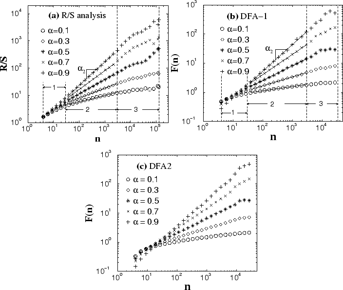
Figure 14:
Scaling behavior of noise with the scaling exponent
. The length of noise
. (a)
Rescaled range analysis (R/S) (b) Order 1 detrended fluctuation analysis
(DFA-1) (c) Order 2 detrended fluctuation analysis. We do the linear
fitting for R/S analysis and DFA-1 in three regions as shown and get
, and for estimated , which are
listed in the Table IV and Table V. We find that
the estimation of is different in the different region.
Before doing that, we want to briefly review the algorithm of R/S
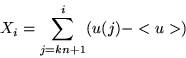
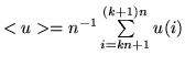
analysis. For a signal (
), it is divided into boxes of equal size . In each box,
the cumulative departure, (for -th box,
), is calculated
(25)
where
, and the rescaled range is defined by
(26)
where
is the standard deviation in each box.
The average of rescaled range in all the boxes of equal size , is obtained and denoted by .
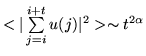
Repeat the above computation over different box size to provide a relationship between and . According to Hurst's experimental
study[64], a power-law relation between and the box size indicates the presence of scaling:
.
Figure 14 shows the results of R/S, DFA-1 and DFA-2 on the
same generated noises. Loosely speaking, we can see that (for
DFA) and (for R/S analysis) show power-law relation with as
expected:
and
. In addition,
there is no significant difference between the results of different
order DFA except for some vertical shift of the curves and the little
bend-down for small box size . The bent-down for very small box of
from higher order DFA is because there are more variables to fit
those few points.
Table IV: Estimated of correlation noise from R/S analysis in
three regions as shown in Fig.14(a). is the input
value of the scaling exponent, is the estimated in the region
1 for , in the region 2 for and
in the region 3 for
. Noise are the same
as used in Table V.
0.1
0.44
0.23
0.12
0.3
0.52
0.37
0.23
0.5
0.62
0.52
0.47
0.7
0.72
0.70
0.45
0.9
0.81
0.87
0.63
Table V: Estimated of correlation noise from DFA-1 in
three regions as shown in Fig.14(b). is the
input value of the scaling exponent, is the estimated in
the region 1 for , in the region 2 for
and in the region 3 for
.
0.1
0.28
0.15
0.08
0.3
0.40
0.31
0.22
0.5
0.55
0.50
0.35
0.7
0.72
0.69
0.55
0.9
0.91
0.91
0.69
Ideally, when analyzing a standard noise, (DFA) and (
analysis) will be a power-law function with a given power: , no
matter which region of and is chosen for calculation.
However, a careful study shows that the scaling exponent depends
on scale . The estimated is different for the different
regions of and as illustrated by Figs. 14(a)
and 14(b) and by Tables IV and V.
It is very important to know the best fitting region of DFA and R/S
analysis in the study of real signals. Otherwise, the wrong
will be obtained if an inappropriate region is selected.
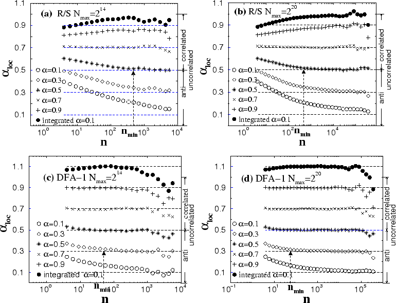
In order to find the best region, we first determine the dependence of
the locally estimated ,
, on
the scale . First, generate a standard noise
with given scaling exponent ; then calculate (or ),
and obtain
by local fitting of
(or ). Same random simulation is repeated 50 times for both
DFA and R/S analysis. The resultant average
, respectively, are illustrated in Fig.15 for DFA-1
and R/S analysis.
If a scaling analysis method is working properly, then the result
from simulation with would
be a horizontal line with slight fluctuation centered about
. Note from
Fig.15 that such a horizontal behavior does not hold
for all the scales but for a certain range from
to
. In
addition, at small scale, R/S analysis gives
if and
if , which has been pointed out by
Mandelbrot[65] while DFA gives
if and
if .
It is clear that the smaller the
and the
larger the
, the better the method. We also
perceive that the expected horizontal behavior stops because
the fluctuations become larger due to the under-sampling of or
when gets closer to the length of the signal
. Furthermore, it can be seen from
Fig.15 that
independent of (if the
best fit region exists), which is why one tenth of the signal length is
the maximum box size when using DFA or R/S analysis.
Figure 15:
The estimated from local fit (a) R/S analysis, the
length of signal
. (b)R/S analysis,
. (c) DFA-1,
(d) DFA-1,
.
come from the average of
simulations. If a technique is working, then the data for scaling
exponent should be a weakly fluctuating horizontal line
centered about
. Note that
such a horizontal behavior does not hold for all the scales. Generally,
such a expected behavior begins from some scale
, holds for a range and ends at a larger scale
. For DFA-1,
is
quite small . For R/S analysis,
is small only when
.
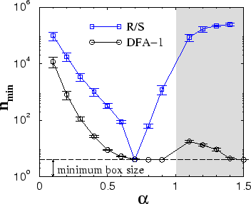
On the contrary,
does not depend on the
since
at small hardly changes as
varies but
it does depend on . Thus, we obtain
quantitatively as shown in Fig.16. For R/S analysis, only for
,
is small; for
a little away from (for example, 0.5),
becomes very large and close to
, indicating that the best fit region will
vanish and R/S analysis does not work at all. Comparing to R/S, DFA
works better since
is quite small for
correlated signals.
Figure 16:
The starting point of good fit region,
,
for
DFA-1 and R/S analysis. The results are obtained from 50 simulations, in
which the length of noise is
. The
condition for a good fit is
. The data for shown in the shading
area are obtained by applying analysis on the integrations of noises
with . It is clear that DFA-1 works better than R/S analysis
because its
is always smaller than that of
R/S analysis.
One problem remains for DFA,
for small
() is still too large comparing to those for large
(). We can improve it by applying DFA on the integration
of the noise with . The resultant new expected
for the integrated signal would be
, while the
for the integrated signal becomes much
smaller as shown also in Fig.16(shading area ). Therefore, for a noise with , it is best to
estimate the scaling exponent of the integrated signal
first and then obtain by
. This is what
we did in the following sections to those anticorrelated signals.
Next:Superposition law for DFA Up:Appendix Previous:Appendix
Zhi Chen
2002-08-28
 . By default, a generated noise has standard deviation
 , and the rescaled range
 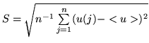 is the standard deviation in each box.
The average of rescaled range in all the boxes of equal size
is the standard deviation in each box.
The average of rescaled range in all the boxes of equal size