A Brief Overview of Multifractal Time Series

Part 2: Using wavelets to detect singular behavior

In a signal with fractal features, an immediate question one faces is "how to quantify the fractal properties of such a signal?'' The first problem is to find the set of locations of the singularities {t_i}, and to estimate the value of h for each t_i.

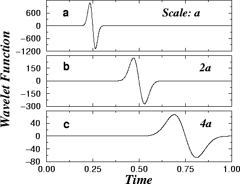
Figure 2: Wavelet function at different scales and positions. We consider as the wavelet function the first derivative of the Gaussian and plot it (a) centered at position b = 0.25 and at scale a = 0.015, (b) centered at position b = 0.5 and at scale 2a, and (c) centered at position b = 0.75 and at scale 4a. Note that the wavelet takes values significantly different from zero just for small ranges.

In contrast to the Fourier transform, which assumes that the signal is stationary at the time scales of interest, the wavelet transform instead determines the frequency content of a signal as a function of time (1). In the Fourier transform, one determines the coefficients that best approximate a function f(t) as a sum of sines and cosines. Similarly, in the wavelet transform, one approximates a function f(t) as a sum of properly weighted basis functions. The basis in the wavelet transform are functions that, like the sines or cosines, can be considered at different frequency but, unlike the sines or cosines, are localized in time and hence have to be translated along the signal. An example of a wavelet basis is the set of functions (see Fig. 2)

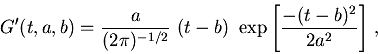(eqn. 3)

where G'(t,a,b) is the first derivative of the Gaussian function, a is an inverse frequency and b is the time location. One determines the coefficients of the wavelet transform by convolving f(t) with G'(t,a,b).

Besides being naturally suited to handle nonstationary signals, the wavelet transform easily removes polynomial contributions that would otherwise mask singular (fractal) behavior. To illustrate this fact, consider a signal f(t) that one can expand for t close to t_i as a series of the form of Eqn. (2). In a fractal analysis, one wants to measure h_i, but for small values of t - t_i, the "trends'' (t - t_i) ^k with k < h_i will dominate the sum. Hence, one ideally wants to remove all terms (t - t_i) ^k for which k < h_i. By convolving f(t) with an appropriate wavelet function, one can put to zero all coefficients that would arise from such polynomial contributions. For instance, the derivative of order k of the Gaussian convolves to zero all polynomial terms up to order k - 1.

Figure 3 shows the wavelet decomposition of a heart rate signal for a healthy subject. The self-similar "arch''-like structures in the figure indicate maxima of the modulus of the wavelet transform. They indicate the time locations (at each scale) of the singularities in the signal. The figure helps illustrate two points. First, the singularities are not present for all times. Second, the location of the singularities, as a function of scale and time, have a fractal structure.

Figure 3: Wavelet decomposition of heart rate signal for healthy subject. Top: Interbeat interval, in second, plotted against beat number for beats 1600 to 3400. Bottom: Modulus of the wavelet decomposition of the signal. The color code is displayed in the color bar at the bottom of the figure. Dark regions correspond to the maxima discussed in the text. The horizontal axis indicates beat number and the vertical axis indicates the "scale" of the wavelet (from 2 to 80 beats). A horizontal cut through the figure reveals the fluctuations on a specific time-scale. The analyzing wavelet used in this decomposition is the second derivative of the Gaussian. Note the fractal structure of maxima (and minima). Continuous maxima line from small scales to large scales determine the time of the singularity at different scales. Merging maxima lines indicate that at scales larger than the merging scale the singularities are no longer isolated. (Courtesy of Plamen Ch. Ivanov.)

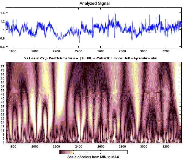
Another interesting property of the wavelet transform is that the coefficients at these maxima---which are a small fraction of the total number of coefficients---are enough to encode the information contained in the signal (3). Moreover, as one follows a maxima line from the lowest scale to higher and higher scales, one is following the same singularity. This fact allows for the calculation of h_i by a power law fit to the coefficients of the wavelet transform along the maxima line (5).

We ask the question "what comes out of our analysis of the signal?" The first possibility is that we find a single value h_i = H for all singularities t_i, the signal is then said to be monofractal (6, 7). The second, more complex, possibility is that we find several distinct values for h, the signal is then said to be multifractal (8, 9).


Previous: Part 1: Fractal behavior in time series	Next: Part 3: The fractal dimension of the singular behavior