Part 3: The fractal dimension of the singular behavior
The next problem is to quantify the "frequency" in the signal of a particular value h of the singularity exponents hi. Let us first assume that our signal is monofractal. Different possibilities can be considered. For example, the set of times with singular behavior {ti} may be a finite fraction of the time series and homogeneously distributed over the signal. But {ti} may also be an asymptotically infinitesimal fraction of the entire signal and have a very heterogeneous structure. That is, the set {ti} may be a fractal itself. In either case, it is useful to quantify the properties of the sets of singularities in the signal by calculating their fractal dimensions (8).
Consider the signal in Fig. 4. This type of signal is usually called a Devil's staircase because it takes constant values except at a subset of points where it changes discontinuously (2, 4). At those points, the function f(t) has singularities. Moreover, all singularities are of the same type --i.e., the signal is monofractal.
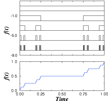
Because the signal of Fig. 4 is deterministic, we can easily identify the position of the singularities. Their positions are shown in the top panel of Fig. 4. One can see that the singularity points arise from the iteration of a Cantor set rule. The signal in the bottom panel of Fig. 4 arises from integrating the "dust'' generated by the Cantor rule (8).
One can easily calculate the fractal dimension of the Cantor set of singularities by using box counting methods. The fractal dimension is, as usual, given by the relation
The signals in Figs. 1a,c are also monofractal. They are usually called fractional Brownian motion. For the signal in Fig. 1a we have h = -0.8 while for the signal in Fig. 1c we have h = 0.2. But in contrast with the devil's staircase of Fig. 4, for which singularities appear only for a very small and heterogeneous set of times, singularities appear uniformly throughout the signals in Figs. 1a,c. Hence, the fractal dimension of the set of singularities is one, the dimension of a line.
| Previous: Part 2: Using wavelets to detect singular behavior |