Part 5: What one learns from the singularity spectra of multifractal signals
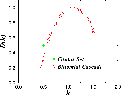
The singularity spectrum D(h) quantifies the degree of nonlinearity in the processes generating the output f(t) in a very compact way (see Fig. 7). For a linear fractal process the output of a system will have the same fractal properties (i.e., the same type of singularities) regardless of initial conditions or of driving forces. In contrast, nonlinear fractal processes will generate outputs with different fractal properties that depend on the input conditions or the history of the system. That is, the output of the system over extended periods of time will display different types of singularities.
| Previous: Part 4: The singularity spectra of multifractal signals | |