|
Part 4: The singularity spectra of multifractal
signals
Our analysis becomes more complex if instead of a single type of singularity,
the signal of interest has multiple types of singularities. As
an example, consider the signal in Fig. 5
which is also a Devil's staircase (i.e., Fig. 4) because
of its many singularities.
But in contrast to the signal of Fig. 4, the types of singularities
vary considerably. The reason for this variation is made clear by the
top panel in Fig. 5. The type of fluctuations in local increments
vary considerably even for the fourth iteration.
|
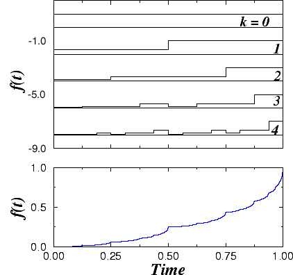 Figure 5: A multifractal Devil's staircase.
Top: Four iteration steps in the building of a multiplicative binomial
cascade. The set is generated by partitioning the mass of the segment
into two parts of equal length but un-equal densities. For the case shown,
the left half of the segment receives 1/4th of the mass while the
right half receives 3/4th of the mass. Bottom: One can generate
a Devil's staircase type of signal by integrating the set generated according
to the previous rule. Such a signal is shown in this panel. Note the presence
of numerous cusp-like features in the signal. These cusps indicate the
times where singularities occur. Because of the local variations in the
mass distribution of the binomial cascade of the Top panel, the singularities
in this case are of several different types.
Figure 5: A multifractal Devil's staircase.
Top: Four iteration steps in the building of a multiplicative binomial
cascade. The set is generated by partitioning the mass of the segment
into two parts of equal length but un-equal densities. For the case shown,
the left half of the segment receives 1/4th of the mass while the
right half receives 3/4th of the mass. Bottom: One can generate
a Devil's staircase type of signal by integrating the set generated according
to the previous rule. Such a signal is shown in this panel. Note the presence
of numerous cusp-like features in the signal. These cusps indicate the
times where singularities occur. Because of the local variations in the
mass distribution of the binomial cascade of the Top panel, the singularities
in this case are of several different types. |
To quantify the variation in the local singularities of the signal of
Fig. 5, we calculate the value of h at every singularity.
Figure 6 shows the signal again and also, by a color coding, the
value of h. Clearly hi can take many different
values. Moreover, by focusing on a single color, i.e., a single
value of h, one can uncover the fractal structure of the corresponding
set of singularities. |
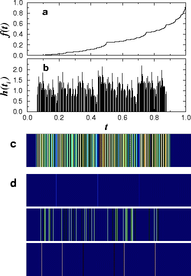 Figure 6: Singularity decomposition of the
multiplicative binomial process of Fig. 5. (a) Devil staircase
after 9 iterations. (b) Position and value of the different singularities
for the signal in (a). (c) Color coding of (b). The dark blue background
indicates absence of singularities. The color spectrum goes from dark
blue to green to yellow and to reddish brown. Blue indicates small values
of h while reddish brown indicates large values of h. Note
that no singularities appear at the edges because we
do not enforce periodic boundary conditions on the signal and hence
cannot perform calculations close to the edges. (d) Decomposition
of the singularities into different sets corresponding to different values
of h. The top panel displays singularities with values of h
approximately two standard deviations smaller than the mean h = 0.6.
The middle panel displays singularities with the average h = 1.1.
Finally, the bottom panel displays singularities with values of h
approximately two standard deviations larger than the mean h = 1.6.
(Note: The color panels in (d) have bars of a single color, unfortunately
color and resolution conflicts may give rise to bars of different colors.)
Figure 6: Singularity decomposition of the
multiplicative binomial process of Fig. 5. (a) Devil staircase
after 9 iterations. (b) Position and value of the different singularities
for the signal in (a). (c) Color coding of (b). The dark blue background
indicates absence of singularities. The color spectrum goes from dark
blue to green to yellow and to reddish brown. Blue indicates small values
of h while reddish brown indicates large values of h. Note
that no singularities appear at the edges because we
do not enforce periodic boundary conditions on the signal and hence
cannot perform calculations close to the edges. (d) Decomposition
of the singularities into different sets corresponding to different values
of h. The top panel displays singularities with values of h
approximately two standard deviations smaller than the mean h = 0.6.
The middle panel displays singularities with the average h = 1.1.
Finally, the bottom panel displays singularities with values of h
approximately two standard deviations larger than the mean h = 1.6.
(Note: The color panels in (d) have bars of a single color, unfortunately
color and resolution conflicts may give rise to bars of different colors.)
|