DFA-1 on noise with sinusoidal trend

In this section, we study how the sinusoidal trend affects the scaling behavior of noise with different type of correlations. We apply the DFA-1 method to a signal which is a superposition of correlated noise with a sinusoidal trend. We observe that there are typically three crossovers in the rms fluctuation $F_{\rm\eta S}(n)$ at characteristic scales denoted by $n_{1\times }$, $n_{2\times }$ and $n_{3\times }$ [Fig. 6]. These three crossovers divide $F_{\rm\eta S}(n)$ into four regions, as shown in Fig. 6(a) (the third crossover cannot be seen in Fig. 6(b) because its scale $n_{3\times }$ is greater than the length of the signal). We find that the first and third crossovers at scales $n_{1\times }$ and $n_{3\times }$ respectively [see Fig. 6] result from the competition between the effects on $F_{\rm\eta S}(n)$ of the sinusoidal signal and the correlated noise. For $n < n_{1\times }$ (region I) and $n > n_{3\times }$ (region IV), we find that the noise has the dominating effect ( $F_{\rm\eta}(n)>F_{\rm S}(n)$), so the behavior of $F_{\rm\eta S}(n)$ is very close to the behavior of $F_{\rm\eta }(n)$ [Eq. (10)]. For $n_{1\times} < n < n_{2\times}$ (region II) and $n_{2\times } < n < n_{3\times }$ (region III) the sinusoidal trend dominates ( $F_{\rm S}(n)>F_{\rm\eta}(n)$), thus the behavior of $F_{\rm\eta S}(n)$ is close to $F_{\rm S}(n)$ [see Fig. 6 and Fig. 7].

Figure 6: Crossover behavior of the root mean square fluctuation function $F_{\rm \eta \rm S}(n)$ (circles) for correlated noise (of length $N_{max}=2^{17}$) with a superposed sinusoidal function characterized by period $T=128$ and amplitude $A_{\rm S} = 2$. The rms fluctuation function $F_{\rm \eta}(n)$ for noise (thick line) and $F_{\rm S}(n)$ for the sinusoidal trend (thin line) are shown for comparison. (a) $F_{\rm \eta \rm S}(n)$ for correlated noise with $\alpha =0.9$. (b) $F_{\rm \eta \rm S}(n)$ for anticorrelated noise with $\alpha =0.9$. There are three crossovers in $F_{\rm \eta \rm S}(n)$, at scales $n_{1\times }$, $n_{2\times }$ and $n_{3\times }$ (the third crossover can not be seen in (b) because it occurs at scale larger than the length of the signal). For $n < n_{1\times }$ and $n > n_{3\times }$, the noise dominates and $F_{\rm \eta \rm S}(n) \approx F_{\rm \eta}(n)$ while for $n_{1\times } < n < n_{3\times }$, the sinusoidal trend dominates and $F_{\rm \eta \rm S}(n) \approx F_{\rm S}(n)$. The crossovers at $n_{1\times }$ and $n_{3\times }$ are due to the competition between the correlated noise and the sinusoidal trend [see Fig. 7], while the crossover at $n_{2\times }$ relates only to the period $T$ of the sinusoidal [Eq. (11)].

Figure 7: Comparison of the detrended fluctuation function for noise, $Y_{\rm \eta}(i)$ and noise with sinusoidal trend, $Y_{\rm \eta S}(i)$ in four regions as shown in Fig. 6. The same signals as in Fig. 6 are used. Panels (a)-(f) correspond to Fig. 6(b) for anticorrelated noise with exponent $\alpha =0.1$, and panels (g)-(h) correspond to the Fig. 6(a) for correlated noise with exponent $\alpha =0.9$. (a)-(b) For all scales $n < n_{1\times }$, the effect of the trend is not pronounced and $Y_{\rm \eta \rm S}(i) \approx Y_{\rm \eta}(i)$ leading to $F_{\rm \eta S}(n) \approx F_{\rm \eta}(n)$ (Fig. 6(a)). (c)(d) For $n_{2\times }> n > n_{1\times }$, the trend is dominant, $Y_{\rm \eta S}(i) \gg Y_{\rm \eta}(i)$ and $F_{\rm \eta S}(n)\approx F_{\rm S}(n)$. Since $n_{2\times } \approx T/2$ (Eq. (11)), the scale $n < T/2$ and the sinusoidal behavior can be approximated as a linear trend. This explains the quadratic background in $Y_{\rm \eta S}(i)$ (d) [see Fig. 2(c)(d)]. (e)(f) For $n_{2\times } < n < n_{3\times }$ (i.e. $n\gg T/2$), the sinusoidal trend again dominates -- $Y_{\rm \eta S}(i)$ is periodic function with period $T$. (g)(h) for $n~>~n_{3\times}$, the effect of the noise is dominant and the scaling of $F_{\rm \eta S}$ follows the scaling of $F_{\rm \eta}$ (Fig. 6(a)).

To better understand why there are different regions in the behavior of $F_{\rm\eta \rm S}(n)$, we consider the detrended fluctuation function [Eq. (3) and Appendix 7.2] of the correlated noise $Y_{\rm\eta }(i)$, and of the noise with sinusoidal trend $Y_{\rm\eta S}$. In Fig. 7 we compare $Y_{\rm\eta }(i)$ and $Y_{\rm\eta S}(i)$ for anticorrelated and correlated noise in the four different regions. For very small scales $n < n_{1\times }$, the effect of the sinusoidal trend is not pronounced, $Y_{\rm \eta S}(i) \approx Y_{\rm\eta}(i)$, indicating that in this scale region the signal can be considered as noise fluctuating around a constant trend which is filtered out by the DFA-1 procedure [Fig. 7(a)(b)]. Note, that the behavior of $Y_{\rm\eta S}$ [Fig. 7(b)] is identical to the behavior of $Y_{\rm\eta L}$ [Fig. 2(b)], since both a sinusoidal with a large period $T$ and a linear trend with small slope $A_{\rm L}$ can be well approximated by a constant trend for $n < n_{1\times }$. For small scales $n_{1\times} < n < n_{2\times}$ (region II), we find that there is a dominant quadratic background for $Y_{\rm\eta S}(i)$ [Fig. 7(d)]. This quadratic background is due to the integration procedure in DFA-1, and is represented by the detrended fluctuation function of the sinusoidal trend $Y_{\rm S}(i)$. It is similar to the quadratic background observed for linear trend $Y_{\rm\eta L}(i)$ [Fig. 2(d)] -- i.e. for $n_{1\times} < n < n_{2\times}$ the sinusoidal trend behaves as a linear trend and $Y_{\rm S}(i) \approx Y_{\rm L}(i)$. Thus in region II the ``linear trend'' effect of the sinusoidal is dominant, $Y_{\rm S}> Y_{\rm\eta}$, which leads to $F_{\rm\eta S}(n)\approx F_{\rm S}(n)$. This explains also why $F_{\rm\eta S}(n)$ for $n < n_{2\times }$ (Fig. 6) exhibits crossover behavior similar to the one of $F_{\rm\eta L}(n)$ observed for noise with a linear trend. For $n_{2\times } < n < n_{3\times }$ (region III) the sinusoidal behavior is strongly pronounced [Fig. 7(f)], $Y_{\rm S}(i) \gg Y_{\rm \eta}(i)$, and $Y_{\rm\eta S}(i) \approx Y_{\rm S}(i)$ changes periodically with period equal to the period of the sinusoidal trend $T$. Since $Y_{\rm\eta S}(i)$ is bounded between a minimum and a maximum value, $F_{\rm\eta S}(n)$ cannot increase and exhibits a flat region (Fig. 6). At very large scales, $n > n_{3\times }$, the noise effect is again dominant ($Y_{\rm S}(i)$ remains bounded, while $Y_{\rm\eta }$ grows when increasing the scale) which leads to $F_{\rm\eta S}(n) \approx F_{\rm\eta }(n)$, and a scaling behavior corresponding to the scaling of the correlated noise.

Figure 8: Dependence of the three crossovers in $F_{\rm \eta S}(n)$ for noise with a sinusoidal trend (Fig. 6) on the period $T$, and amplitude $A_{\rm S}$ of the sinusoidal trend. (a) Power-law relation between the first crossover scale $n_{1\times }$ and the period $T$ for fixed amplitude $A_{\rm S}$ and varying correlation exponent $\alpha$: $n_{1\times} \sim T^{\theta_{\rm T1}}$, where $\theta_{\rm T1}$ is a positive crossover exponent [see Table II and Eq. 14]. (b) Power-law relation between the first crossover $n_{1\times }$ and the amplitude of the sinusoidal trend $A_{\rm S}$ for fixed period $T$ and varying correlation exponent $\alpha$: $n_{1\times} \sim A_{\rm S}^{\theta_{\rm A1}}$ where $\theta_{\rm A1}$ is a negative crossover exponent [Table II and Eq. (14)]. (c) The second crossover scale $n_{2\times }$ depends only on the period $T$: $n_{2\times} \sim T^{\theta_{\rm T2}}$, where $\theta_{\rm T2}\approx 1$. (d) Power-law relation between the third crossover $n_{3\times }$ and $T$ for fixed amplitude $A_{\rm S}$ and varying $\alpha$ trend: $n_{3\times} \sim T^{\theta_{\rm T3} }$. (e) Power-law relation between the third crossover $n_{3\times }$ and $A_{\rm S}$ for fixed $T$ and varying $\alpha$: $n_{3\times} \sim \left(A_{\rm S}\right)^{\theta_{A3} }$. We find that $\theta_{\rm A3}=\theta_{\rm T3}$ [Table III and Eq. (15)].

First, we consider $n_{1\times }$. Surprisingly, we find that for noise with any given correlation exponent $\alpha$ the crossover scale $n_{1\times }$ exhibits long-range power-law dependence of the period $T$ -- $n_{1\times } \sim T^{\theta _{\rm T1}}$, and the amplitude $A_{\rm S}$ -- $n_{1\times} \sim \left(A_{\rm S}\right)^{\theta_{\rm A1}}$ of the sinusoidal trend [see Fig. 8(a) and (b)]. We find that the "crossover exponents" $\theta _{\rm T1}$ and $\theta _{\rm A1}$ have the same magnitude but different sign -- $\theta _{\rm T1}$ is positive while $\theta _{\rm A1}$ is negative. We also find that the magnitude of $\theta _{\rm T1}$ and $\theta _{\rm A1}$ increases for the larger values of the correlation exponents $\alpha$ of the noise. We present the values of $\theta _{\rm T1}$ and $\theta _{\rm A1}$ for different correlation exponent $\alpha$ in Table II. To understand these power-law relations between $n_{1\times }$ and $T$, and between $n_{1\times }$ and $A_{\rm S}$, and also how the crossover scale $n_{1\times }$ depends on the correlation exponent $\alpha$ we employ the superposition rule [Eq. 10] and estimate $n_{1\times }$ analytically as the first intercept $n_{1\times}^{th}$ of $F_{\rm\eta }(n)$ and $F_{\rm S}(n)$. From Eqs. (12) and (6), we obtain the following dependence of $n_{1\times }$ on $T$, $A_{\rm S}$ and $\alpha$:

$$n_{1\times} = \left(\frac{b_0}{k_1} \frac{T}{A_{\rm S}}\right)^{1/(2 - \alpha)}$$ (14)

From this analytical calculation we obtain the following relation between the two crossover exponents $\theta _{\rm T1}$ and $\theta _{\rm A1}$ and the correlation exponent $\alpha$: $\theta_{\rm T1}~=~-~\theta_{\rm A1}~=~1/{(2-\alpha)}$, which is in a good agreement with the observed values of $\theta _{\rm T1}$, $\theta _{\rm A1}$ obtained from simulations [see Fig. 8(a) (b) and Table II].

Next, we consider $n_{2\times }$. Our analysis of the rms fluctuation function $F_{\rm S}(n)$ for the sinusoidal signal in Fig. 5 suggests that the crossover scale $F_{\rm S}(n)$ does not depend on the amplitude $A_{\rm S}$ of the sinusoidal. The behavior of the rms fluctuation function $F_{\rm\eta S}(n)$ for noise with superimposed sinusoidal trend in Fig. 6(a) and (b) indicates that $n_{2\times }$ does not depend on the correlation exponent $\alpha$ of the noise, since for both correlated ($\alpha =0.9$) and anticorrelated ($\alpha=0$) noise ($T$ and $A_{\rm S}$ are fixed), the crossover scale $n_{2\times }$ remains unchanged. We find that $n_{2\times }$ depends only on the period $T$ of the sinusoidal trend and exhibits a long-range power-law behavior $n_{2\times } \sim T^{\theta _{\rm T2}}$ with a crossover exponent $\theta _{\rm T2}\approx 1$ (Fig. 8(c)) which is in agreement with the prediction of Eq.(11).

For the third crossover scale $n_{3\times }$, as for $n_{1\times }$ we find a power-law dependence on the period $T$, $n_{3\times} \sim T^{\theta_{T3}}$, and amplitude $A_{\rm S}$, $n_{3\times } \sim \left (A_{\rm S}\right )^{\theta _{A3} }$,of the sinusoidal trend [see Fig. 8(d) and (e)]. However, in contrast to the $n_{1\times }$ case, we find that the crossover exponents $\theta_{\rm Tp3}$ and $\theta_{\rm A3}$ are equal and positive with decreasing values for increasing correlation exponents $\alpha$. In Table III, we present the values of these two exponents for different correlation exponent $\alpha$. To understand how the scale $n_{3\times }$ depends on $T$, $A_{\rm S}$ and the correlation exponent $\alpha$ simultaneously, we again employ the superposition rule [Eq. (10)] and estimate $n_{3\times }$ as the second intercept $n_{3\times}^{th}$ of $F_{\rm\eta }(n)$ and $F_{\rm S}(n)$. From Eqs. (13) and (6), we obtain the following dependence:

$$n_{3\times} = \left (\frac{1}{2 \sqrt{2} \pi b_0} A_{\rm S} T \right)^{1/\alpha}.$$ (15)

From this analytical calculation we obtain $\theta_{\rm T3}=\theta_{\rm A3} = 1/\alpha$ which is in good agreement with the values of $\theta_{\rm T3}$ and $\theta_{\rm A3}$ observed from simulations [Table III].

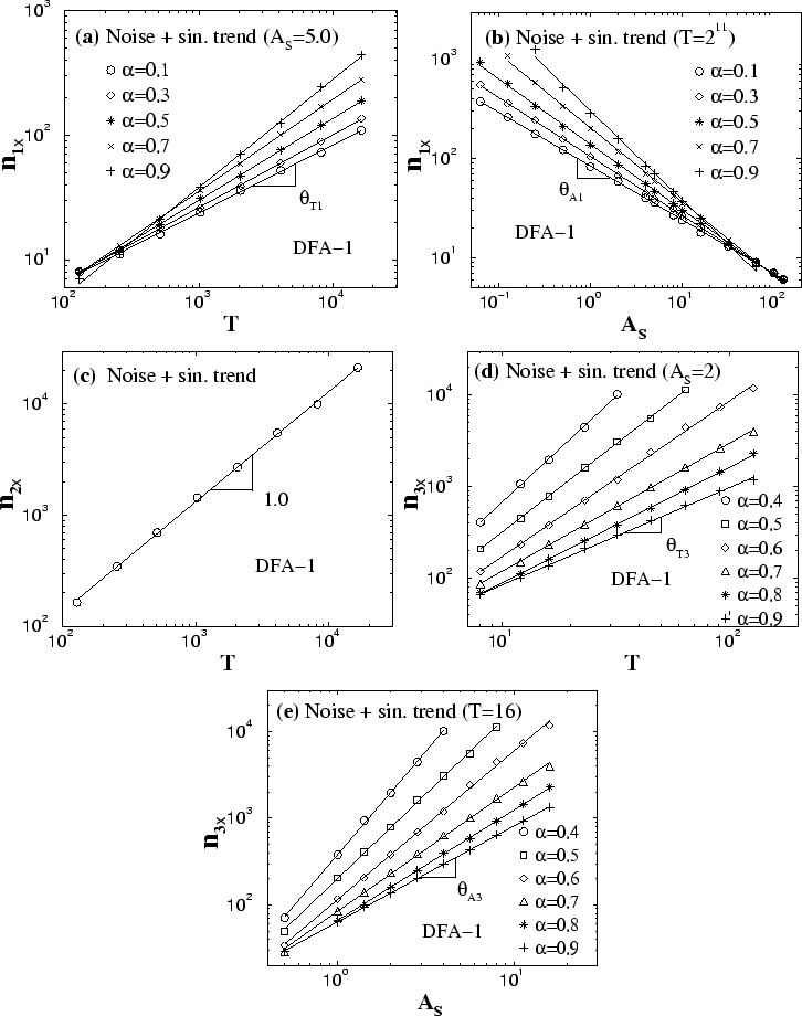
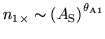
Table II: The crossover exponents $\theta _{\rm T1}$ and $\theta _{\rm A1}$ characterizing the power-law dependence of $n_{1\times }$ on the period $T$ and amplitude $A_{\rm S}$ obtained from simulations: $n_{1\times } \sim T^{\theta _{\rm T1}}$ and $n_{1\times} \sim \left(A_{\rm S}\right)^{\theta_{\rm A1}}$ for different value of the correlation exponent $\alpha$ of noise [Fig. 8(a)(b)]. The values of $\theta _{\rm T1}$ and $\theta _{\rm A1}$ are in good agreement with the analytical predictions $\theta_{\rm T1}=-\theta_{\rm A1}=1/(2-\alpha)$ [Eq. (14)].

$\alpha$	$\theta _{\rm T1}$	- $\theta _{\rm A1}$	$1/(2-\alpha)$
0.1	0.55	0.54	0.53
0.3	0.58	0.59	0.59
0.5	0.66	0.66	0.67
0.7	0.74	0.75	0.77
0.9	0.87	0.90	0.91

Table III: The crossover exponents $\theta_{\rm T3}$ and $\theta_{\rm A3}$ for the power-law relations: $n_{3\times } \sim T^{\theta _{\rm T3} }$ and $n_{3\times} \sim \left(A_{\rm S}\right)^{\theta_{\rm A3}}$ for different value of the correlation exponent $\alpha$ of noise [Fig. 8(c)(d)]. The values of $\theta_{p3}$ and $\theta_{a3}$ obtained from simulations are in good agreement with the analytical predictions $\theta_{\rm T3}=\theta_{\rm A3} = 1/\alpha$ [Eq. (15)].

$\alpha$	$\theta_{\rm T3}$	$\theta_{\rm A3}$	$1/\alpha$
0.4	2.29	2.38	2.50
0.5	1.92	1.95	2.00
0.6	1.69	1.71	1.67
0.7	1.39	1.43	1.43
0.8	1.26	1.27	1.25
0.9	1.06	1.10	1.11

Finally, our simulations show that all three crossover scales $n_{1\times }$, $n_{2\times }$ and $n_{3\times }$ do not depend on the length of the signal $N_{max}$, since $F_{\rm\eta }(n)$ and $F_{\rm S}(n)$ do not depend on $N_{max}$ as shown in Eqs. (6), (10), (12), and (13).