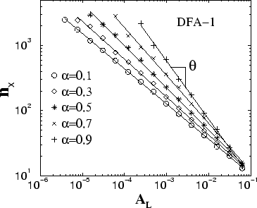
Table I: The crossover exponent  from the power-law relation between the
crossover scale from the power-law relation between the
crossover scale  and the slope of the linear trend and the slope of the linear trend  --
--
 --for different values
of the correlation exponents --for different values
of the correlation exponents  of the noise
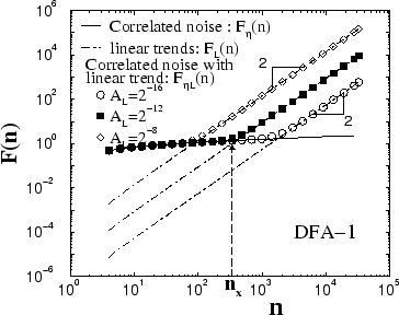
[Fig. 3]. The values of obtained from our
simulations are in good agreement with the analytical prediction of the noise
[Fig. 3]. The values of obtained from our
simulations are in good agreement with the analytical prediction
 [Eq. (9)]. Note that are not always
exactly equal to because [Eq. (9)]. Note that are not always
exactly equal to because
 in simulations is not a
perfect simple power-law function and the way we determine numerically
is just approximated. in simulations is not a
perfect simple power-law function and the way we determine numerically
is just approximated.
|
|
|
| 0.1 |
-0.54 |
-0.53 |
| 0.3 |
-0.58 |
-0.59 |
| 0.5 |
-0.65 |
-0.67 |
| 0.7 |
-0.74 |
-0.77 |
| 0.9 |
-0.89 |
-0.91 |
|