DFA-1 on Quadratic trend

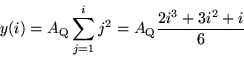
Let us suppose now a series of the type $u(i)=A_{\rm Q} i^{2}$. The integrated time series $y(i)$ is

$$y(i)=A_{\rm Q}\sum_{j=1}^{i}j^{2}=A_{\rm Q}\frac{2i^{3}+3i^{2}+i}{6}$$ (38)

As before, let us call $N_{max}$ and $n$ the sizes of the series and box, respectively. The rms fluctuation function $F_{\rm Q}(n)$ measuring the rms fluctuation is now defined as

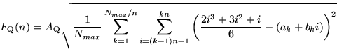$$F_{\rm Q}(n)=A_{\rm Q}\sqrt{\frac{1}{N_{max}}\sum_{k=1}^{N_... ...\left(\frac{2i^{3}+3i^{2}+i}{6}-(a_{k}+b_{k}i)\right) ^{2} }$$ (39)

where $a_{k}$ and $b_{k}$ are the parameters of a least-squares fit of the $k$-th box of size $n$. As before, $a_{k}$ and $b_{k}$ can be determined analytically, thus giving:

$$a_{k}=\frac{1}{15}n^{3}+n^{3}k^{2}-\frac{7}{15}n^{3}k+\frac... ...ac{2}{3}k^{3}n^{3}-\frac{1}{2}n^{2}k^{ 2}+%% \frac{1}{15}kn$$ (40)

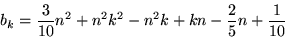$$b_{k}=\frac{3}{10}n^{2}+n^{2}k^{2}-n^{2}k+kn-\frac{2}{5}n+\frac{1}{10}$$ (41)

Once $a_{k}$ and $b_{k}$ are known, $F(n)$ can be evaluated, giving:

$$F_{\rm Q}(n)=A_{\rm Q}\allowbreak \frac{1}{1260}\sqrt{-21\l... ...ght) \left( 32n^{2}-6n-81-210N_{max}-140N_{max}^{2}\right) }$$ (42)

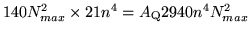As $N_{max}>n$, the dominant term inside the square root is given by $140N_{max}^{2}\times 21n^{4}=A_{\rm Q}\allowbreak 2940n^{4}N_{max}^{2}$, and then one has approximately

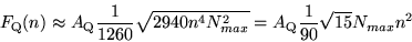$$F_{\rm Q}(n)\approx A_{\rm Q} \frac{1}{1260}\sqrt{2940n^{4}N_{max}^{2}}=A_{\rm Q}\frac{1}{90}\sqrt{15}N_{max}n^{2}$$ (43)

leading directly to an exponent 2 in the DFA analysis. An interesting consequence derived from Eq. (43) is that, $F_{\rm Q}(n)$ depends on the length of signal $N_{max}$, and the DFA line ( $\log F_{\rm Q}(n)$ vs $\log n$) for quadratic series $u(i)=A_{\rm Q} i^{2}$ of different $N_{max}$ does not overlap (as is the case for linear trends).