Signals with different local correlations

Next we consider nonstationary signals which consist of segments with identical standard deviation ($\sigma =1$) but different correlations. We obtain such signals using the following procedure: (1) we generate two stationary signals $u_{1}(i)$ and $u_{2}(i)$ (see Sec. 2) of identical length $N_{max}$ and with different correlations, characterized by scaling exponents $\alpha_{1}$ and $\alpha_{2}$; (2) we divide the signals $u_{1}(i)$ and $u_{2}(i)$ into non-overlapping segments of size $W$; (3) we randomly replace a fraction $p$ of the segments in signal $u_{1}(i)$ with the corresponding segments of $u_{2}(i)$. In Fig. 5(a), we show an example of such a complex nonstationary signal with different local correlations. In this Section, we study the behavior of the r.m.s. fluctuation function $F(n)/n$. We also investigate $F(n)/n$ separately for each component of the nonstationary signal (which consists only of the segments with identical local correlations) and suggest an approach, based on the DFA results, to recognize such complex structures in real data.

Figure 5: Scaling behavior of a nonstationary signal with two different scaling exponents. (a) Nonstationary signal (length $N_{max}=2^{20}$, standard deviation $\sigma =1$) which is a mixture of correlated segments with exponent $\alpha _{1}=0.1$ (90% of the signal) and segments with exponent $\alpha _{2}=0.9$ (10% of the signal). The segment size is $W=20$; (b) the 90% component containing all segments with $\alpha _{1}=0.1$ and the remaining segments (with $\alpha _{2}=0.9$) are replaced by zero; (c) the 10% component containing all segments with $\alpha _{2}=0.9$ and the remaining segments (with $\alpha _{1}=0.1$) are replaced by zero; (d) DFA results for the mixed signal in (a), for the individual components in (b) and (c), and our prediction obtained from the superposition rule.

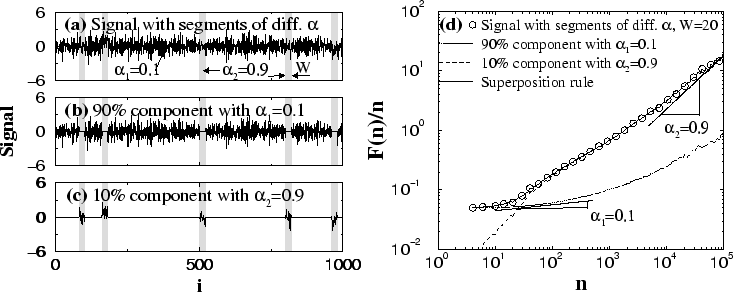In Fig. 5(d), we present the DFA result on such a nonstationary signal, composed of segments with two different types of local correlations characterized by exponents $\alpha _{1}=0.1$ and $\alpha _{2}=0.9$. We find that at small scales, the slope of $F(n)/n$ is close to $\alpha_{1}$ and at large scales, the slope approaches $\alpha_{2}$ with a bump in the intermediate scale regime. This is not surprising, since $\alpha_{1}<\alpha_{2}$ and thus $F(n)/n$ is bound to have a small slope ($\alpha_{1}$) at small scales and a large slope ($\alpha_{2}$) at large scales. However, it is surprising that although 90% of the signal consists of segments with scaling exponent $\alpha_{1}$, $F(n)/n$ deviates at small scales ($n\approx 10$) from the behavior expected for an anti-correlated signal $u(i)$ with exponent $\alpha_{1}$ [see, e.g., the solid line in Fig. 2(b)]. This suggests that the behavior of $F(n)/n$ for a nonstationary signal comprised of mixed segments with different correlations is dominated by the segments exhibiting higher positive correlations even in the case when their relative fraction in the signal is small. This observation is pertinent to real data such as: (i) heart rate recordings during sleep where different segments corresponding to different sleep stages exhibit different types of correlations[33]; (ii) DNA sequences including coding and non-coding regions characterized by different correlations[5,8,16] and (iii) brain wave signals during different sleep stages[62].

To better understand the complex behavior of $F(n)/n$ for such nonstationary signals, we study their components separately. Each component is composed only of those segments in the original signal which are characterized by identical correlations, while the segments with different correlations are substituted with zeros [see Figs. 5(b) and (c)]. Since the two components of the nonstationary signal in Fig. 5(a) are independent, based on the superposition rule [Eq. (5)], we expect that the r.m.s. fluctuation function $F(n)/n$ will behave as $\sqrt{[F_1(n)/n]^2+[F_2(n)/n]^2}$, where $F_1(n)/n$ and $F_2(n)/n$ are the r.m.s. fluctuation functions of the components in Fig. 5(b) and Fig. 5(c), respectively. We find a remarkable agreement between the superposition rule prediction and the result of the DFA method obtained directly from the mixed signal [Fig 5(d)]. This finding helps us understand the relation between the scaling behavior of the mixed nonstationary signal and its components.

Information on the effect of such parameters as the scaling exponents $\alpha_{1}$ and $\alpha_{2}$, the size of the segments $W$ and their relative fraction $p$ on the scaling behavior of the components provides insight into the scaling behavior of the original mixed signal. When the original signal comes from real data, its composition is a priori unknown. A first step is to ``guess'' the type of correlations (exponents $\alpha_{1}$ and $\alpha_{2}$) present in the signal, based on the scaling behavior of $F(n)/n$ at small and large scales [Fig 5(d)]. A second step is to determine the parameters $W$ and $p$ for each component by matching the scaling result from the superposition rule with the original signal. Hence in the following subsections, we focus on the scaling properties of the components and how they change with $p$, $\alpha$ and $W$.