Dependence on the fraction of segments

First, we study how the correlation properties of the components depend on the fraction $p$ of the segments with identical local correlations.

For components containing segments with anti-correlations ($0<\alpha<0.5$) and fixed size $W$ [Fig. 5(b)], we find a crossover to random behavior ($\alpha =0.5$) at large scales, which becomes more pronounced (shift to smaller scales) when the fraction $p$ decreases [Fig. 6(a)]. At small scales ($n\leq W$), the slope of $F(n)/n$ is identical to that expected for a stationary signal $u(i)$ (i.e., $p=1$) with the same anti-correlations [solid line in Fig. 6(a)]. Moreover, we observe a vertical shift in $F(n)/n$ to lower values when the fraction $p$ of non-zero anti-correlated segments decreases. We find that at small scales after rescaling $F(n)/n$ by $\sqrt {p}$, all curves collapse on the curve for the stationary anti-correlated signal $u(i)$ [Fig. 6(a)]. Since at small scales ($n\leq W$) the behavior of $F(n)/n$ does not depend on the segment size $W$, this collapse indicates that the vertical shift in $F(n)/n$ is due only to the fraction $p$. Thus, to determine the fraction $p$ of anti-correlated segments in a nonstationary signal [mixture of anti-correlated and correlated segments, Fig. 5(a)] we only need to estimate at small scales the vertical shift in $F(n)/n$ between the mixed signal [Fig. 5(d)] and a stationary signal $u(i)$ with identical anti-correlations. This approach is valid for nonstationary signals where the fraction $p$ of the anti-correlated segments is much larger than the fraction of the correlated segments in the mixed signal [Fig. 5(a)], since only under this condition the anti-correlated segments can dominate $F(n)/n$ of the mixed signal at small scales [Fig. 5(d)].

Figure 6: Dependence of the scaling behavior of components on the fraction $p$ of the segments with identical local correlations, emphasizing data collapse at small scales. The segment size is $W=20$ and the length of the components is $N_{max}=2^{20}$. (a) Components containing anti-correlated segments ($\alpha =0.1$), at small scales ($n\leq W$). The slope of $F(n)/n$ is identical to that expected for a stationary ($p=1$) signal with the same anti-correlations. After rescaling $F(n)/n$ by $\sqrt {p}$, at small scales all curves collapse on the curve for the stationary anti-correlated signal. (b) Components containing correlated segments ($\alpha =0.9$), at small scales ($n\leq W$). The slope of $F(n)/n$ is identical to that expected for a stationary ($p=1$) signal with the same correlations. After rescaling $F(n)/n$ by $\sqrt {p}$, at small scales all curves collapse on the curve for the stationary correlated signal.

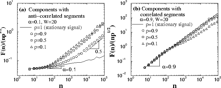For components containing segments with positive correlations ($0.5<\alpha<1$) and fixed size $W$ [Fig. 5(c)], we observe a similar behavior for $F(n)/n$, with collapse at small scales ($n\leq W$) after rescaling by $\sqrt {p}$ [Fig. 6(b)] (For $\alpha>1$, there are exceptions with different rescaling factors, see Appendix 7.2). At small scales the values of $F(n)/n$ for components containing segments with positive correlations are much larger compared to the values of $F(n)/n$ for components containing an identical fraction $p$ of anti-correlated segments [Fig. 6(a)]. Thus, for a mixed signal where the fraction of correlated segments is not too small (e.g., $p\geq 0.2$), the contribution at small scales of the anti-correlated segments to $F(n)/n$ of the mixed signal [Fig. 5(d)] may not be observed, and the behavior (values and slope) of $F(n)/n$ will be dominated by the correlated segments. In this case, we must consider the behavior of $F(n)/n$ of the mixed signal at large scales only, since the contribution of the anti-correlated segments at large scales is negligible. Hence, we next study the scaling behavior of components with correlated segments at large scales.

For components containing segments with positive correlations and fixed size $W$ [Fig. 5(c)], we find that at large scales the slope of $F(n)/n$ is identical to that expected for a stationary signal $u(i)$ (i.e., $p=1$) with the same correlations [solid line in Fig. 7(a)]. We also observe a vertical shift in $F(n)/n$ to lower values when the fraction $p$ of non-zero correlated segments in the component decreases. We find that after rescaling $F(n)/n$ by $p$, at large scales all curves collapse on the curve representing the stationary correlated signal $u(i)$ [Fig. 7(a)]. Since at large scales ($n\gg W$), the effect of the zero segments of size $W$ on the r.m.s. fluctuation function $F(n)/n$ for components with correlated segments is negligible, even when the zero segments are 50% of the component [see Fig. 7(a)], the finding of a collapse at large scales indicates that the vertical shift in $F(n)/n$ is only due to the fraction $p$ of the correlated segments. Thus, to determine the fraction $p$ of correlated segments in a nonstationary signal (which is a mixture of anti-correlated and correlated segments [Fig. 5(a)]), we only need to estimate at large scales the vertical shift in $F(n)/n$ between the mixed signal [Fig. 5(d)] and a stationary signal $u(i)$ with identical correlations.

Figure 7: Dependence of scaling behavior of components on the fraction $p$ of the segments with identical local correlations, emphasizing data collapse at large scales. The segment size is $W=20$ and the length of the components is $N_{max}=2^{20}$. (a) Components containing correlated segments ($\alpha =0.9$), at large scales ($n\gg W$). The slope of $F(n)/n$ is identical to that expected for a stationary ($p=1$) signal with the same correlations. After rescaling $F(n)/n$ by $p$, at large scales all curves collapse on the curve for the stationary correlated signal. (b) Components containing anti-correlated segments ($\alpha =0.1$), at large scales ($n\gg W$). There is a crossover to random behavior ($\alpha =0.5$). After rescaling $F(n)/n$ by $\sqrt {p(1-p)}$, all curves collapse at large scales.

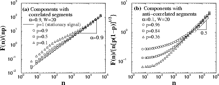For components containing segments with anti-correlations and fixed size $W$ [Fig. 5(b)], we find that at large scales in order to collapse the $F(n)/n$ curves ($n\gg W$) [Fig. 6(a)] we need to rescale $F(n)/n$ by $\sqrt {p(1-p)}$ [see Fig. 7(b)]. Note that there is a difference between the rescaling factors for components with anti-correlated and correlated segments at small [Figs. 6(a-b)] and large [Figs. 7(a-b)] scales. We also note that for components with correlated segments ($\alpha >0.5$) and sufficiently small $p$, there is a different rescaling factor of $\sqrt {p(1-p)}$ in the intermediate scale regime [see Appendix 7.2, Fig. 10].

For components containing segments of white noise ($\alpha =0.5$), we find no change in the scaling exponent as a function of the fraction $p$ of the segments, i.e., $\alpha =0.5$ for the components at both small and large scales. However, we observe at all scales a vertical shift in $F(n)/n$ to lower values with decreasing $p$: $F(n)/n \sim \sqrt{p}$.