Signals with different local standard deviations

Figure 4: Scaling behavior of nonstationary correlated signals with different local standard deviation. (a) Anti-correlated signal ($\alpha =0.1$) with standard deviation $\sigma _1=1$ and amplified segments with standard deviation $\sigma _2=4$. The size of each segment is $W=20$ and the fraction of the amplified segments is $p=0.1$ from the total length of the signal ( $N_{max}=2^{20}$). (b) Scaling behavior of the signal in (a) for a different fraction $p$ of the amplified segments (after normalization of the globe standard deviation to unity). A crossover from anti-correlated behavior ($\alpha =0.1$) at small scales to random behavior ($\alpha =0.5$) at large scales is observed. (c) Dependence of the crossover scale $n_{\times }$ on the fraction $p$ of amplified segments for the signal in (a). $n_{\times }$ is determined from the difference $\Delta$ of $\log_{10}[F(n)/n]$ between the nonstationary signal with amplified segments and the original stationary signal. Here we choose $\Delta =0.04$. (d) Scaling behavior of nonstationary signals obtained from correlated stationary signals ($1>\alpha >0.5$) with standard deviation $\sigma _1=1$, for a different fraction of the amplified segments with $\sigma _2=4$. No difference in the scaling is observed, compared to the original stationary signal.

Here we consider nonstationary signals comprised of segments with the same local scaling exponent, but different local standard deviations. We first generate a stationary correlated signal $u(i)$ (see Sec. 2) with fixed standard deviation $\sigma _1=1$. Next, we divide the signal $u(i)$ into non-overlapping segments of size $W$. We then randomly choose a fraction $p$ of the segments and amplify the standard deviation of the signal in these segments, $\sigma _2=4$ [Fig.4(a)]. Finally, we normalize the entire signal to global standard deviation $\sigma =1$ by dividing the value of each point of the signal by $\sqrt{(1-p)\sigma_1^2+p\sigma_2^2}$.

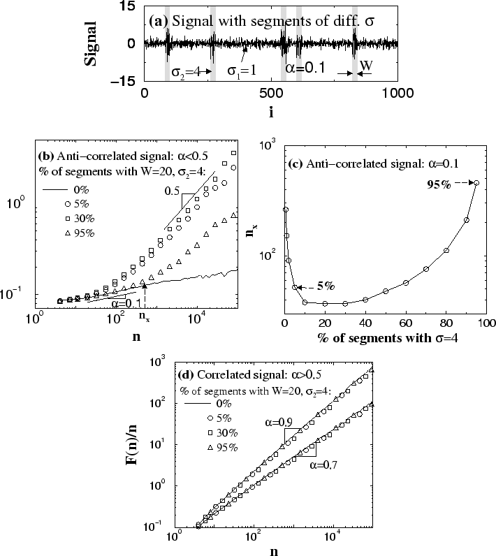
For nonstationary anti-correlated signals ($\alpha <0.5$) with segments characterized by two different values of the standard deviation, we observe a crossover at scale $n_{\times }$ [Fig.4(b)]. For small scales $n<n_{\times }$, the behavior is anti-correlated with an exponent equal to the scaling exponent $\alpha$ of the original stationary anti-correlated signal $u(i)$. For large scales $n>n_{\times }$, we find a transition to random behavior with exponent $0.5$, indicating that the anti-correlations have been destroyed. The dependence of crossover scale $n_{\times }$ on the fraction $p$ of segments with larger standard deviation is shown in Fig. 4(c). The dependence is not monotonic because for $p=0$ and $p=1$, the local standard deviation is constant throughout the signal, i.e., the signal becomes stationary and thus there is no crossover. Note the asymmetry in the value of $n_{\times }$ -- a much smaller value of $n_{\times }$ for $p=0.05$ compared to $p=0.95$ [see Fig. 4(b-c)]. This result indicates that very few segments with a large standard deviation (compared to the rest of the signal) can have a strong effect on the anti-correlations in the signal. Surprisingly, the same fraction of segments with a small standard deviation (compared to the rest of the signal) does not affect the anti-correlations up to relatively large scales.

For nonstationary correlated signals ($\alpha >0.5$) with segments characterized by two different values of the standard deviation, we surprisingly find no difference in the scaling of $F(n)/n$, compared to the stationary correlated signals with constant standard deviation [Fig. 4(d)]. Moreover, this observation remains valid for different sizes of the segments $W$ and for different values of the fraction $p$ of segments with larger standard deviation. We note that in the limiting case of very large values of $\sigma_{2}/\sigma_{1}$, when the values of the signal in the segments with standard deviation $\sigma_{1}$ could be considered close to ``zero'', the results in Fig. 4(d) do not hold and we observe a scaling behavior similar to that of the signal in Fig. 5(c) (see following section).