A simplified and general definition characterizes a time series as stationary if its mean, standard deviation and higher moments, as well as the correlation functions, are invariant under time translation. Signals that do not obey these conditions are nonstationary. As discussed above, a bounded time series can be mapped to a self-similar process by integration; for example, a sequence of coin flips can be mapped in this way to a one-dimensional random walk (see this tutorial for more on this subject, including hands-on experiments), a stationary integrated time series. Another challenge facing investigators applying this type of fractal analysis to physiologic time series, however, is that they are often highly nonstationary (Fig. 1a). The integration procedure will make the nonstationarity of the original data even more apparent.
To overcome this complication, we have introduced a modified root mean square analysis of a random walk, termed detrended fluctuation analysis ( DFA) [11, 12], which may be applied to the analysis of biological data. Among the advantages of DFA over conventional methods (e.g., spectral analysis and Hurst analysis) are that it permits the detection of intrinsic self-similarity embedded in a seemingly nonstationary time series, and also avoids the spurious detection of apparent self-similarity, which may be an artifact of extrinsic trends. This method has been successfully applied to a wide range of simulated and physiologic time series in recent years [11, 12, 13, 14, 15, 16].
Please note that although the DFA algorithm works well for certain types of nonstationary time series (especially slowly varying trends), it is not designed to handle all possible nonstationarities in real-world data.
To illustrate the DFA algorithm, we use the interbeat time series shown in
Fig. 3a as an example. First, the interbeat
interval time series (of total length N) is integrated, ![]() , where
B(i) is the i-th interbeat interval and
, where
B(i) is the i-th interbeat interval and ![]() is the
average interbeat interval. As discussed above, this integration step maps the
original time series to a self-similar process. Next we measure the vertical
characteristic scale of the integrated time series. To do so, the integrated
time series is divided into boxes of equal length, n. In each box of
length n, a least squares line is fit to the data (representing the
trend in that box) (Fig. 4). The
y coordinate of the straight line segments is denoted by
is the
average interbeat interval. As discussed above, this integration step maps the
original time series to a self-similar process. Next we measure the vertical
characteristic scale of the integrated time series. To do so, the integrated
time series is divided into boxes of equal length, n. In each box of
length n, a least squares line is fit to the data (representing the
trend in that box) (Fig. 4). The
y coordinate of the straight line segments is denoted by ![]() . Next
we detrend the integrated time series, y(k), by subtracting the
local trend,
. Next
we detrend the integrated time series, y(k), by subtracting the
local trend, ![]() , in each box. For a given box
size n, the characteristic size of fluctuation for this integrated and
detrended time series is calculated by
, in each box. For a given box
size n, the characteristic size of fluctuation for this integrated and
detrended time series is calculated by
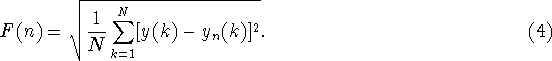
(This
quantity F is similar but not identical to the quantity s
measured in the previous section.)
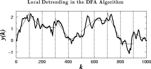
Figure 4:
The integrated time series: ![]() , where B(i) is
the interbeat interval shown in Fig. 3(a). The
vertical dotted lines indicate boxes of size n=100, and the solid
straight line segments represent the ``trend'' estimated in each box by a
linear least-squares fit.
, where B(i) is
the interbeat interval shown in Fig. 3(a). The
vertical dotted lines indicate boxes of size n=100, and the solid
straight line segments represent the ``trend'' estimated in each box by a
linear least-squares fit.
This computation is repeated over all time scales (box sizes) to provide a
relationship between F(n) and the box size n. Typically,
F(n) will increase with box size n. A linear relationship
on a double log graph indicates the presence of scaling (self-similarity)--the
fluctuations in small boxes are related to the fluctuations in larger boxes in
a power-law fashion. The slope of the line relating log F(n) to
log n determines the scaling exponent (self-similarity parameter), ![]() ,
as discussed previously.
,
as discussed previously.