For a self-similar process with ![]() , the fluctuations grow with
the window size in a power-law way. Therefore, the fluctuations on
large observation windows are exponentially larger than those of
smaller windows. As a result, the time series is unbounded.
However, for most physiologic time series of interest, such as
heart rate and gait, are bounded--they cannot have arbitrarily
large amplitudes no matter how long the data set is. This practical
restriction causes further complications for our analyses. Consider
the case of the heart rate time series shown in Fig. 3a. If
we zoom in on a subset of the time series, we notice an apparently
self-similar pattern. To visualize this self-similarity, we do not
need to rescale the y-axis (
, the fluctuations grow with
the window size in a power-law way. Therefore, the fluctuations on
large observation windows are exponentially larger than those of
smaller windows. As a result, the time series is unbounded.
However, for most physiologic time series of interest, such as
heart rate and gait, are bounded--they cannot have arbitrarily
large amplitudes no matter how long the data set is. This practical
restriction causes further complications for our analyses. Consider
the case of the heart rate time series shown in Fig. 3a. If
we zoom in on a subset of the time series, we notice an apparently
self-similar pattern. To visualize this self-similarity, we do not
need to rescale the y-axis (![]() )--only rescaling the x-axis is
needed. Therefore, according to Eq. 3, the self-similarity
parameter is 0--not an informative result. Consider another example
where we randomize the sequential order of the original heart rate
time series generating a completely uncorrelated ``control'' time
series (Fig. 3b)--white noise. The white noise data set also
has a self-similarity parameter of 0. However, it is obvious that the
patterns in Figs. 3a and b are quite different. An immediate problem, therefore, is how to distinguish the trivial parameter 0 in the latter case of
uncorrelated noise, from the non-trivial parameter 0 computed for the
original data.
)--only rescaling the x-axis is
needed. Therefore, according to Eq. 3, the self-similarity
parameter is 0--not an informative result. Consider another example
where we randomize the sequential order of the original heart rate
time series generating a completely uncorrelated ``control'' time
series (Fig. 3b)--white noise. The white noise data set also
has a self-similarity parameter of 0. However, it is obvious that the
patterns in Figs. 3a and b are quite different. An immediate problem, therefore, is how to distinguish the trivial parameter 0 in the latter case of
uncorrelated noise, from the non-trivial parameter 0 computed for the
original data.
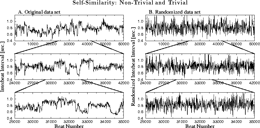
Figure:
A cardiac inter-heartbeat interval (inverse of heart rate) time series
is shown in (A) and a randomized control is shown in (B). Successive
magnifications of the sub-sets show that both time series are
self-similar with a trivial exponent ![]() (i.e.,
(i.e., ![]() ),
albeit the patterns are very different in (A) and (B).
),
albeit the patterns are very different in (A) and (B).
Physicists and mathematicians have developed an innovative solution for this central problem in time series analysis [8, 9]. The ``trick'' is to study the fractal properties of the accumulated (integrated) time series, rather than those of the original signals [7, 10]. One well-known physical example with relevance to biological time series is the dynamics of Brownian motion. In this case, the random force (noise) acting on particles is bounded, similar to physiologic time series. However, the trajectory (an integration of all previous forces) of the Brownian particle is not bounded and exhibits fractal properties that can be quantified by a self-similarity parameter. When we apply fractal scaling analysis to the integrated time series of Figs. 3a and b, the self-similarity parameters are indeed different in these two cases, providing meaningful distinctions between the original and the randomized control data sets. The details of this analysis will be discussed in the next section.
In summary, mapping the original bounded time series to an integrated signal is a crucial step in fractal time series analysis. In the rest of this chapter, therefore, we apply fractal analysis techniques after integration of the original time series.