Before describing the metrics we use to quantitatively characterize the fractal properties of heart rate and gait dynamics, we first review the meaning of the term fractal. The concept of a fractal is most often associated with geometrical objects satisfying two criteria: self-similarity and fractional dimensionality. Self-similarity means that an object is composed of sub-units and sub-sub-units on multiple levels that (statistically) resemble the structure of the whole object [7]. Mathematically, this property should hold on all scales. However, in the real world, there are necessarily lower and upper bounds over which such self-similar behavior applies. The second criterion for a fractal object is that it have a fractional dimension. This requirement distinguishes fractals from Euclidean objects, which have integer dimensions. As a simple example, a solid cube is self-similar since it can be divided into sub-units of 8 smaller solid cubes that resemble the large cube, and so on. However, the cube (despite its self-similarity) is not a fractal because it has an (=3) dimension. (Click here for a hands-on experiment about fractal curves.)
The concept of a fractal structure, which lacks a characteristic length scale, can be extended to the analysis of complex temporal processes. However, a challenge in detecting and quantifying self-similar scaling in complex time series is the following: Although time series are usually plotted on a 2-dimensional surface, a time series actually involves two different physical variables. For example, in Figure 1, the horizontal axis represents ``time,'' while the vertical axis represents the value of the variable that changes over time (in this case, heart rate). These two axes have independent physical units, minutes and beats/minute, respectively. (Even in cases where the two axes of a time series have the same units, their intrinsic physical meaning is still different.) This situation is different from that of geometrical curves (such as coastlines and mountain ranges) embedded in a 2-dimensional plane, where both axes represent the same physical variable. To determine if a 2-dimensional curve is self-similar, we can do the following test: (i) take a subset of the object and rescale it to the same size of the original object, using the same magnification factor for both its width and height; and then (ii) compare the statistical properties of the rescaled object with the original object. In contrast, to properly compare a subset of a time series with the original data set, we need two magnification factors (along the horizontal and vertical axes), since these two axes represent different physical variables.
To put the above discussion into mathematical terms: A time-dependent
process (or time series) is self-similar if
![]()
where ![]() means that the statistical
properties of both sides of the equation are identical. In other
words, a self-similar process, y(t), with a parameter
means that the statistical
properties of both sides of the equation are identical. In other
words, a self-similar process, y(t), with a parameter ![]() has
the identical probability distribution as a properly rescaled process,
has
the identical probability distribution as a properly rescaled process,
![]() , i.e., a time series which has been rescaled on
the x-axis by a factor a (
, i.e., a time series which has been rescaled on
the x-axis by a factor a (![]() ) and on the y-axis by a factor
of
) and on the y-axis by a factor
of ![]() (
(![]() ). The exponent
). The exponent ![]() is
called the self-similarity parameter.
is
called the self-similarity parameter.
In practice, however, it is impossible to determine whether two processes are statistically identical, because this strict criterion requires their having identical distribution functions (including not just the mean and variance, but all higher moments as well). Therefore, one usually approximates this equality with a weaker criterion by examining only the means and variances (first and second moments) of the distribution functions for both sides of Eq. 1.
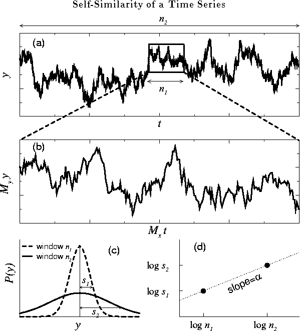
Figure: Illustration of the concept of self-similarity for a
simulated random walk. (a) Two observation windows, with time scales
![]() and
and ![]() , are shown for a self-similar time series y(t). (b)
Magnification of the smaller window with time scale
, are shown for a self-similar time series y(t). (b)
Magnification of the smaller window with time scale ![]() . Note that
the fluctuations in (a) and (b) look similar provided that two
different magnification factors,
. Note that
the fluctuations in (a) and (b) look similar provided that two
different magnification factors, ![]() and
and ![]() , are applied on the
horizontal and vertical scales, respectively. (c) The probability
distribution, P(y), of the variable y for the two windows in (a),
where
, are applied on the
horizontal and vertical scales, respectively. (c) The probability
distribution, P(y), of the variable y for the two windows in (a),
where ![]() and
and ![]() indicate the standard deviations for these two
distribution functions. (d) Log-log plot of the characteristic scales
of fluctuations, s, versus the window sizes, n.
indicate the standard deviations for these two
distribution functions. (d) Log-log plot of the characteristic scales
of fluctuations, s, versus the window sizes, n.
Figure 2a shows an example of a self-similar time series. We note
that with the appropriate choice of scaling factors on the x- and y-axis,
the rescaled time series (Fig. 2b) resembles the original time
series (Fig. 2a). The self-similarity parameter ![]() defined
in Eq. 1 can be calculated by a simple relation
defined
in Eq. 1 can be calculated by a simple relation
![]()
where ![]() and
and ![]() are the appropriate magnification factors along
the horizontal and vertical direction, respectively.
are the appropriate magnification factors along
the horizontal and vertical direction, respectively.
In practice, we usually do not know the value of the ![]() exponent
in advance. Instead, we face the challenge of extracting this scaling
exponent (if one does exist) from a given time series. To this end it
is necessary to study the time series on observation windows with
different sizes and adopt the weak criterion of self-similarity defined
above to calculate the exponent
exponent
in advance. Instead, we face the challenge of extracting this scaling
exponent (if one does exist) from a given time series. To this end it
is necessary to study the time series on observation windows with
different sizes and adopt the weak criterion of self-similarity defined
above to calculate the exponent ![]() . The basic idea is
illustrated in Fig. 2. Two observation windows
(Fig. 2a), window 1 with horizontal size
. The basic idea is
illustrated in Fig. 2. Two observation windows
(Fig. 2a), window 1 with horizontal size ![]() and
window 2 with horizontal size
and
window 2 with horizontal size ![]() , were arbitrarily selected
to demonstrate the procedure. The goal is to find the correct
magnification factors such that we can rescale window 1 to resemble
window 2. It is straightforward to determine the magnification factor
along the horizontal direction,
, were arbitrarily selected
to demonstrate the procedure. The goal is to find the correct
magnification factors such that we can rescale window 1 to resemble
window 2. It is straightforward to determine the magnification factor
along the horizontal direction, ![]() . But for the
magnification factor along the vertical direction,
. But for the
magnification factor along the vertical direction, ![]() , we need to
determine the vertical characteristic scales of windows 1 and 2. One
way to do this is by examining the probability distributions
(histograms) of the variable y for these two observation windows
(Fig. 2c). A reasonable estimate of the characteristic scales
for the vertical heights, i.e., the typical fluctuations of y, can
be defined by using the standard deviations of these two histograms,
denoted as
, we need to
determine the vertical characteristic scales of windows 1 and 2. One
way to do this is by examining the probability distributions
(histograms) of the variable y for these two observation windows
(Fig. 2c). A reasonable estimate of the characteristic scales
for the vertical heights, i.e., the typical fluctuations of y, can
be defined by using the standard deviations of these two histograms,
denoted as ![]() and
and ![]() , respectively. Thus, we have
, respectively. Thus, we have
![]() . Substituting
. Substituting ![]() and
and ![]() into Eq. 2, we
obtain
into Eq. 2, we
obtain
![]()
This relation is simply the slope of the line that joins these two
points, (![]() ,
, ![]() ) and (
) and (![]() ,
, ![]() ), on a log-log plot
(Fig. 2d).
), on a log-log plot
(Fig. 2d).
In analyzing ``real-world'' time series, we perform the above
calculations using the following procedures: (1) For any given size of
observation window, the time series is divided into subsets of
independent windows of the same size. To obtain a more reliable
estimation of the characteristic fluctuation at this window size, we
average over all individual values of s obtained from these subsets.
(2) We then repeat these calculations, not just for two window sizes
(as illustrated above), but for many different window sizes. The
exponent ![]() is estimated by fitting a line on the log-log plot
of s versus n across the relevant range of scales.
is estimated by fitting a line on the log-log plot
of s versus n across the relevant range of scales.