Next: Further work Up: Analyzing Data with WAVE Previous: Using the Scope window
We now turn to an extended example showing how an application can be written in C to be used with WAVE . The application is an example only; it is not intended for any serious application, clinical or otherwise. Its structure illustrates, however, how a real application can be built.
As noted in the previous section, changes in the ST segment of the ECG
are of interest because of their relationship to ischemia
(which occurs when the oxygen supplied by the coronary arteries is
insufficient to meet the demands of the myocardium).
Characteristically, ischemia affects the shape of the ST segment,
which corresponds to the first phase of ventricular repolarization
following the QRS complex; typically, the ECG signal may not return
to its baseline, or isoelectric, level (defined in the interval
between the P-wave and the QRS complex) until after the T-wave. The
level of the ST segment relative to the isoelectric level is the ST
deviation. Conventionally, the ST deviation is measured at a single
point 80 milliseconds after the J point (the end of the QRS complex).
An ST deviation of 100 ![]() V is considered to be clinically
significant, and consistent with ischemia.
V is considered to be clinically
significant, and consistent with ischemia.
We will design a program for measuring ST deviations using WAVE . We
assume that the QRS complexes have been marked, and that, in addition,
two special annotations (`(', signifying the beginning of the QRS
complex, and `)', signifying its end) have also been marked for the
first beat that we wish to measure. (To use our program on an
unannotated record, we can use
![]() , and then
insert the special annotations manually around the first beat.)
, and then
insert the special annotations manually around the first beat.)
Let us begin by deciding how the program should be invoked from WAVE . At a minimum, we should be able to specify which signal should be measured, and the region of interest. The program also needs to know the record and annotator names (the latter so that it can read the annotations it needs to get started). Following the conventions used by many other WFDB applications, we add the following entry to WAVE 's menu file:
Measure ST deviation<TAB>stdev -r $RECORD -a $ANNOTATOR \
                          -f $START -t $END -s $SIGNAL
Here
is the C source for the program. If this looks unfamiliar, read
about how to write WFDB applications in the
WFDB Programmer's Guide.
The source for this program is included in the WAVE distribution as stdev.c. Copy this file to the WAVE host if necessary, and compile it in a terminal window using a command such as
cc -o stdev -O stdev.c -lwfdb
Depending on how the WFDB Software Package has been installed on the
WAVE host, you may need to use -I/usr/local/include and
-L/usr/local/lib options so that the compiler can
locate the *.h files and the WFDB library. On some systems, the
C compiler may have a different name, such as gcc. Consult an
expert such as your system administrator if in doubt about compiling
a C program with the WFDB library.
Once the source has been compiled successfully, install the executable binary file stdev in a directory in your PATH. If you are using the C-shell, you may need to run the command rehash to make your shell aware that the program has been installed. Test the program in the terminal window by typing
stdev
which should produce a brief summary of its options. If this test fails, figure out why and correct the problem before continuing.
Once the program has been compiled and installed successfully, try running it from within WAVE . Remember that the annotation file must include the `(' and `)' annotations to mark the beginning and end of the first beat to be measured. Using it on signal 0 of record 100s, with a suitably augmented set of reference annotations, I obtained output beginning with:
    0.0171296	-84
    0.0306481	-24
    0.0437963	-9
    0.0569907	-34
    0.0701389	-64
    0.08375	-59
    0.0946296	-49
    0.111204	-29
    0.125278	-4
    0.138796	-59
    0.151944	-9
    0.164815	-34
(Your output will vary, depending on the exact locations of the `(' and `)' annotations that you insert.)
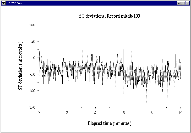
If plt has been installed on your system, you can use it to plot this output (see plt(1), in the WFDB Applications Guide, for details on plt). To do so, modify the entry in the menu file, so that it becomes:
    Plot ST deviation<TAB>stdev -r $RECORD -a $ANNOTATOR \
                            -f $START -t $END -s $SIGNAL | \
                           plt 0 1 \
                            -t "ST deviations, Record $RECORD" \
                            -x "Elapsed time (minutes)" \
                            -y "ST deviation (microvolts)"
If you now reread the menu and use the new
![]() button, plot2d opens a window with a plot in it, similar to
figure 3.5.
button, plot2d opens a window with a plot in it, similar to
figure 3.5.