


Next: Plotting Two or More Data Sets Together
Up: Plotting Data
Previous: Plotting Data
This section contains a series of plots made using many of the plotstyles
described in the previous pages. Each plot was made using the same data
file, styles.data, which contains:
0 0 0 0
1 -1 .25 1
2 -2 .5 2
3 1 .25 1
4 4 1 4
5 1 .25 1
6 -2 .5 2
7 -1 .25 1
8 0 0 0
In several of these examples, the data are plotted in 90% grey, to make clear
how certain plotstyles use the plot color. plt is told to do this by
the ``(G.90)'' appended to the plotstyle specification in each case; see
chapter 11 for details on using color and grey level
definitions such as these.
Figure 6.3:
Produced using the command:
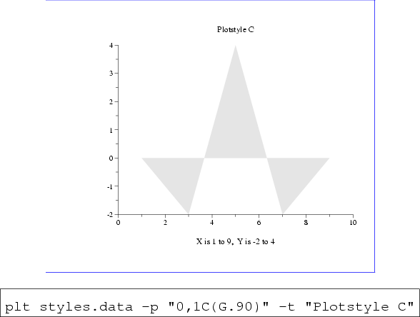 |
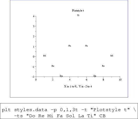
Figure 6.4:
Produced using the command:
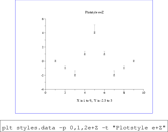 |
Figure 6.5:
Produced using the command:
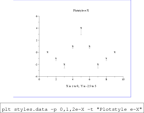 |
Figure 6.6:
Produced using the command:
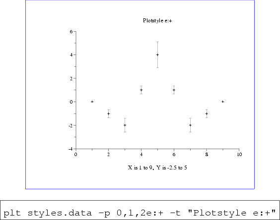 |
Figure 6.7:
Produced using the command:
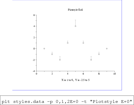 |
Figure 6.8:
Produced using the command:
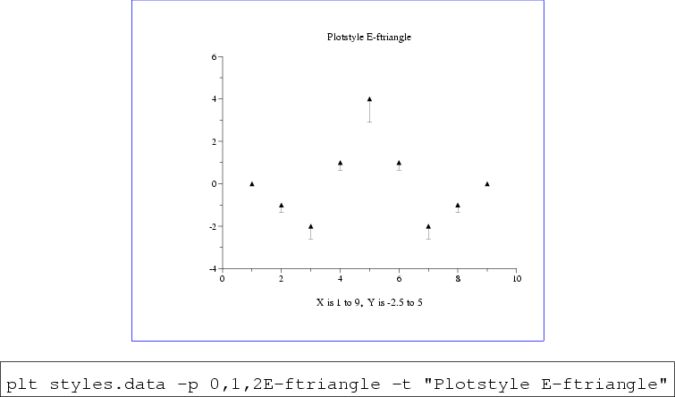 |
Figure 6.9:
Produced using the command:
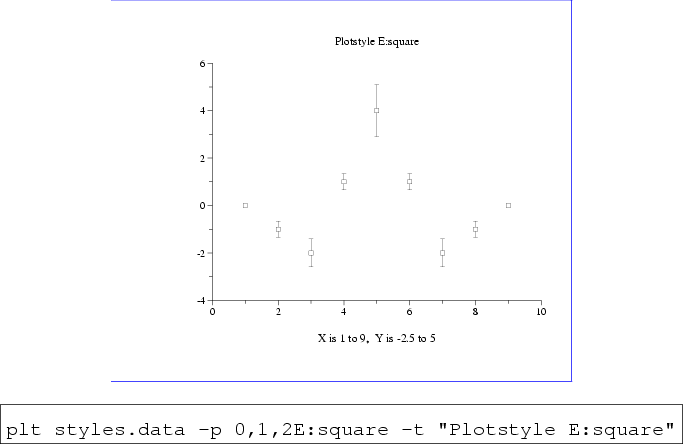 |
Figure 6.10:
Produced using the command:
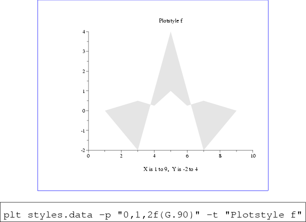 |
Figure 6.11:
Produced using the command:
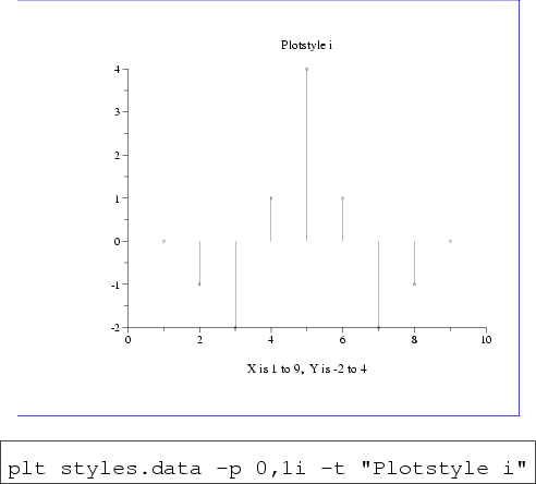 |
Figure 6.12:
Produced using the command:
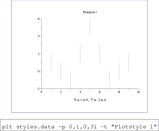 |
Figure 6.13:
Produced using the command:
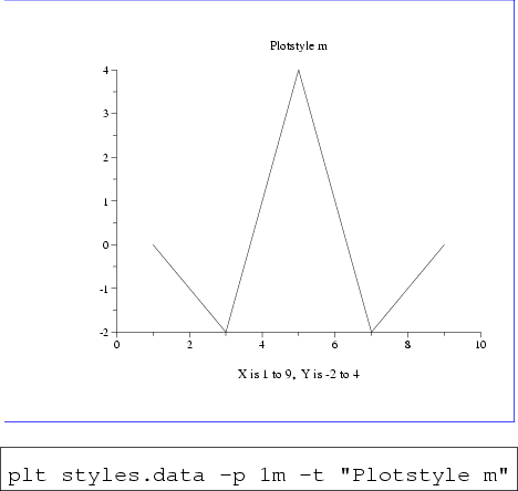 |
Figure 6.14:
Produced using the command:
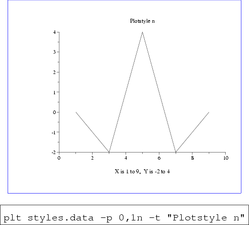 |
Figure 6.15:
Produced using the command:
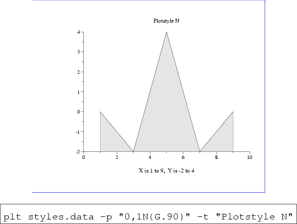 |
Figure 6.16:
Produced using the command:
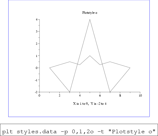 |
Figure 6.17:
Produced using the command:
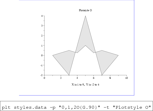 |
Figure 6.18:
Produced using the command:
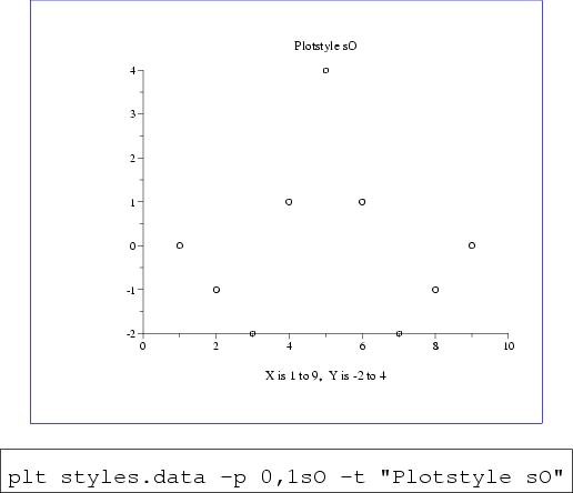 |
Figure 6.19:
Produced using the command:
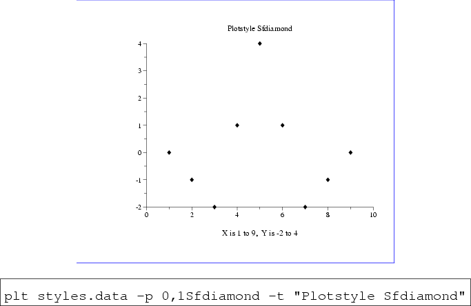 |
Figure 6.20:
Produced using the command:
 |
Next: Plotting Two or More Data Sets Together
Up: Plotting Data
Previous: Plotting Data
George B. Moody (george@mit.edu)
2005-04-26