Approximate Entropy (ApEn)

This description originally appeared in slightly modified form, and without the example, in Ho, Moody, Peng, et al. [4].

is a ``regularity statistic'' that quantifies the unpredictability of fluctuations in a time series such as an instantaneous heart rate time series, . Intuitively, one may reason that the presence of repetitive patterns of fluctuation in a time series renders it more predictable than a time series in which such patterns are absent. reflects the likelihood that ``similar'' patterns of observations will not be followed by additional ``similar'' observations. A time series containing many repetitive patterns has a relatively small ; a less predictable (i.e., more complex) process has a higher .

The algorithm for computing has been published elsewhere [1-4]. Here, we provide a brief summary of the calculations, as applied to a time series of heart rate measurements, . Given a sequence , consisting of instantaneous heart rate measurements , , , , we must choose values for two input parameters, and , to compute the approximate entropy, , of the sequence. The second of these parameters, , specifies the pattern length, and the third, , defines the criterion of similarity. We denote a subsequence (or pattern) of heart rate measurements, beginning at measurement within , by the vector . Two patterns, and , are similar if the difference between any pair of corresponding measurements in the patterns is less than , i.e., if

Now consider the set of all patterns of length [i.e., ], within . We may now define

where is the number of patterns in that are similar to (given the similarity criterion ). The quantity is the fraction of patterns of length that resemble the pattern of the same length that begins at interval . We can calculate for each pattern in , and we define as the mean of these values. The quantity expresses the prevalence of repetitive patterns of length in . Finally, we define the approximate entropy of , for patterns of length and similarity criterion , as

i.e., as the natural logarithm of the relative prevalence of repetitive patterns of length compared with those of length .

Thus, if we find similar patterns in a heart rate time series, estimates the logarithmic likelihood that the next intervals after each of the patterns will differ (i.e., that the similarity of the patterns is mere coincidence and lacks predictive value). Smaller values of imply a greater likelihood that similar patterns of measurements will be followed by additional similar measurements. If the time series is highly irregular, the occurrence of similar patterns will not be predictive for the following measurements, and will be relatively large.

It should be noted that has significant weaknesses, notably its strong dependence on sequence length and its poor self-consistency (i.e., the observation that for one data set is larger than for another for a given choice of and should, but does not, hold true for other choices of and ). For an excellent review of the shortcomings of and the strengths of alternative statistics, see reference [5].

Example:

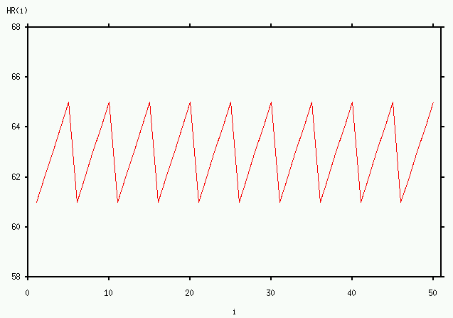
An example may help to clarify the process of calculating . Suppose that , and that the sequence consists of 50 samples of the function illustrated above:

(i.e., the sequence is periodic with a period of 5). Let's choose (this choice simplifies the calculations for this example, but similar results would be obtained for other nearby values of ) and (again, the value of can be varied somewhat without affecting the result). This gives us:

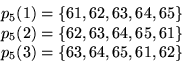
and so on. The first question to be answered is: how many of the are similar to ? Since we have chosen as the similarity criterion, this means that each of the 5 components of must be within units of the corresponding component of . Thus, for example, is not similar to , since their last components (61 and 65) differ by more than 2 units. The conditions for similarity to will be satisfied only by , , , , ..., , as well as by itself [i.e., for 10 of the ], so we have

Since the total number of is ,

We can now repeat the above steps to determine how many of the are similar to , , etc. By the same reasoning, is similar to , , , ..., , so that

and in general

(This last statement is true only for the particular example we are considering, since we have specified a sequence with a period of 5, and we have chosen m = 5 as well.)

Hence is either or , depending on , and the mean value of all 46 of the is:

In order to obtain , we need to repeat all of the calculations above for . Doing so, we obtain:

so that

and . Finally, we calculate that

This is a very small value of ApEn, which suggests that the original time series is highly predictable (as indeed it is).

ApEn Software

In view of the weaknesses in ApEn, and in deference to the wishes of SM Pincus, we do not provide an implementation of ApEn here. This description is provided here so that researchers who wish to use ApEn can write their own code for doing so.

An ApEn implementation in Matlab m-code is included in Danny Kaplan's Software for Heart Rate Variability.

References:

1. Pincus SM. Approximate entropy as a measure of system complexity. Proc Natl Acad Sci USA 1991;88:2297-2301.

2. Pincus SM, Goldberger AL. Physiological time-series analysis: What does regularity quantify? Am J Physiol 1994;266(Heart Circ Physiol):H1643-H1656.

3. Ryan SM, Goldberger AL, Pincus SM, Mietus J, Lipsitz LA. Gender and age-related differences in heart rate dynamics: Are women more complex than men? J Am Coll Cardiol 1994;24:1700-1707.

4. Ho KKL, Moody GB, Peng CK, Mietus JE, Larson MG, Levy D, Goldberger AL. Predicting survival in heart failure case and control subjects by use of fully automated methods for deriving nonlinear and conventional indices of heart rate dynamics. Circulation 1997 (August);96(3):842-848.

5. Richman JS, Moorman JR. Physiological time-series analysis using approximate entropy and sample entropy. Am J Physiol Heart Circ Physiol 278(6):H2039-H2049 (2000).